How Unequal Is It? Measuring New Jersey's Pollution Gap Like Economists Measure Income Inequality

From “is there a gap?” to “how big is it?”

Post after post on this site has found that pollution and environmental hazards in New Jersey fall more heavily on overburdened communities and communities of color: incinerators, power plants, contaminated sites, toxic-release facilities, and chemical accident risk. Each of those posts asked whether a gap exists. This one asks a different question: how unequal is the distribution, and which burdens are the most unequal?

To answer it, I borrowed a tool that economists and public health researchers use to measure inequality in income and health: the concentration curve and concentration index (O’Donnell et al., 2008).

How a concentration curve works

1. Line up all of New Jersey’s residents from those living in the least diverse neighborhoods to those in the most diverse.
2. Walk along the line and keep a running total of the share of all pollution exposure in the state.
3. If pollution were shared equally, the bottom 50% of residents would have 50% of the exposure, and the curve would follow the diagonal line of perfect equality.
4. If pollution is concentrated among residents of more diverse neighborhoods, the curve sags below the diagonal.

The concentration index turns the gap between the curve and the diagonal into one number. 0 means perfectly equal, positive numbers mean exposure is concentrated among residents of more diverse neighborhoods, and the maximum is 1. I weighted every neighborhood by its population, so each person counts equally.

Data

I used the final public version of EPA’s EJScreen (2.32), saved on February 5, 2025, the day EPA removed it (see my EJScreen post). It covers 12 environmental indicators for New Jersey’s 6,524 populated block groups (U.S. EPA, 2024).

Findings

Every indicator is concentrated in more diverse neighborhoods

Indicator	Concentration index by race (95% CI)	By income	Share of statewide exposure borne by the most diverse 20% of residents
Underground storage tanks	0.40 (0.39–0.41)	0.30	44%
Hazardous waste facilities	0.31 (0.30–0.32)	0.15	34%
Traffic	0.27 (0.26–0.28)	0.14	33%
Chemical accident facilities	0.24 (0.23–0.26)	0.16	32%
Superfund sites	0.24 (0.23–0.26)	0.14	31%
Industrial wastewater	0.20 (0.15–0.25)	0.20	30%
Diesel particulate matter	0.16 (0.16–0.17)	0.06	27%
Nitrogen dioxide	0.15 (0.15–0.16)	0.07	28%
Lead paint risk	0.10 (0.09–0.11)	0.06	26%
Toxic air releases	0.07 (0.04–0.10)	0.07	24%
Fine particles (PM2.5)	0.02 (0.02–0.02)	0.01	21%
Ozone	0.01 (0.01–0.01)	0.00	20%

All 12 indicators have a concentration index above zero, and for all 12 the 95% bootstrap confidence interval excludes zero. If burdens were shared equally, the most diverse fifth of residents would bear 20% of each. Instead they bear 44% of the exposure to underground storage tanks, 34% of hazardous waste facility exposure, and about a third of traffic, chemical accident, and Superfund exposure.

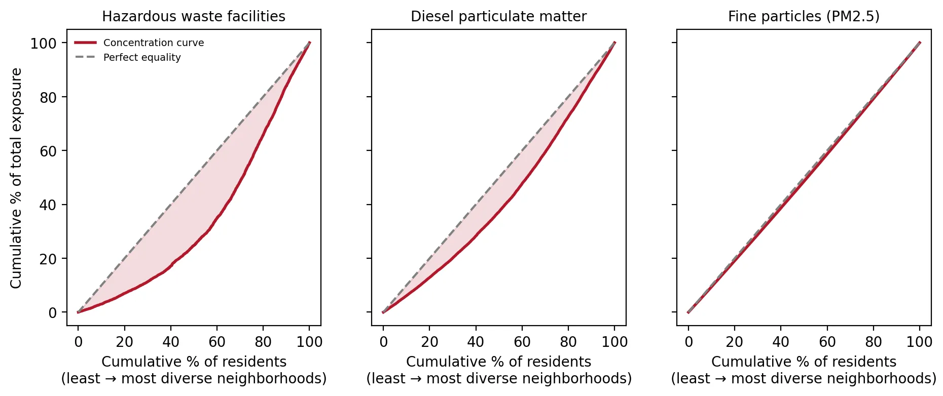Figure 1. Concentration curves show hazardous waste exposure is the most unequal and PM2.5 the least.

The curves show it visually. For hazardous waste facilities, the curve sags far below the line of equality. For diesel exhaust, it sags less but clearly. For PM2.5, which spreads across whole regions, the curve sits just below the line.

Local hazards are the most unequal

The most unequal burdens are local, site-based hazards: storage tanks, hazardous waste, traffic, chemical facilities, and Superfund sites. These stay close to where they’re located, so where facilities and roads were built determines who lives with them. Regional air pollutants like ozone and PM2.5 blow across the state and are spread more evenly, though still not perfectly.

Race matters more than income

Figure 2. Most pollution burdens are more concentrated by race than by income.

For 11 of 12 indicators, pollution is more concentrated by race than by income. Across all 12 combined, the concentration index by race (0.157) is more than twice the index by income (0.071). This matches national research: the 1987 Toxic Wastes and Race report found race was the strongest predictor of where hazardous waste facilities were located (Commission for Racial Justice, 1987), and a 2021 study found that fine-particle pollution disproportionately and systemically affects people of color (Tessum et al., 2021).

Why this matters

Saying “pollution is unequal” is a claim; a concentration index puts a number on it, with an uncertainty range, in a way that can be tracked over time and compared across states and pollutants. These results show that New Jersey’s environmental inequality is real, statistically certain, largest for exactly the facility-based hazards the Environmental Justice Law regulates, and more strongly tied to race than to income.

Limitations

• Neighborhood averages. Each block group is treated as one unit, so inequality within neighborhoods isn’t captured.
• Indicator choice. EJScreen’s indicators are proxies for exposure, not measured doses.
• The bootstrap resamples neighborhoods. It shows the result is stable, but it can’t fix errors in the underlying data.

Code project (Level 6): measuring inequality

Goal: Measure how concentrated each environmental burden is among residents of more diverse and lower-income neighborhoods.

Data: EJScreen 2.32 New Jersey block groups (Internet Archive copy, February 5, 2025); NJDEP OBC data (version effective March 31, 2026).

Steps:

1. Rank all neighborhoods by % people of color (and separately by % low-income), weighted by population.
2. Compute each neighborhood’s fractional rank in the population.
3. Concentration index = 2 × covariance(pollution, rank) ÷ mean pollution (population-weighted).
4. Bootstrap 500 times to get 95% confidence intervals.
5. Draw concentration curves against the line of equality.

def conc_index(x, rank_by, w):
    o = np.argsort(rank_by); x, w = x[o], w[o]
    r = np.cumsum(w) / w.sum() - w / (2 * w.sum())        # fractional rank
    mu = np.average(x, weights=w)
    return 2 * np.average((x - mu) * (r - 0.5), weights=w) / mu

New skills: inequality measurement, population weighting, and bootstrapping a custom statistic.

References

- Commission for Racial Justice, United Church of Christ. (1987). Toxic wastes and race in the United States. https://www.ucc.org/wp-content/uploads/2020/12/ToxicWastesRace.pdf
- O'Donnell, O., van Doorslaer, E., Wagstaff, A., & Lindelow, M. (2008). Analyzing health equity using household survey data (Chapter 8: The concentration index). World Bank. https://openknowledge.worldbank.org/handle/10986/6896
- Tessum, C. W., Paolella, D. A., Chambliss, S. E., Apte, J. S., Hill, J. D., & Marshall, J. D. (2021). PM2.5 polluters disproportionately and systemically affect people of color in the United States. Science Advances, 7(18), eabf4491. https://doi.org/10.1126/sciadv.abf4491
- U.S. Environmental Protection Agency. (2024). EJScreen 2.32 block group data with state percentiles [Data set; Internet Archive copy of February 5, 2025]. https://web.archive.org/web/20250205213739/https://gaftp.epa.gov/ejscreen/2024/2.32_August_UseMe/EJSCREEN_2024_BG_StatePct_with_AS_CNMI_GU_VI.csv.zip
- New Jersey Department of Environmental Protection. (2026). Environmental Justice (EJ) Law Combined Stressor Summary (Current) [Data set]. https://www.arcgis.com/home/item.html?id=8f1eeb5074d147af8ab3e5e5a4f72d2b